Sampling

Code for Quiz 11.

1. Load the R package we will use.

library(tidyverse)
library(moderndive)

Question:

7.2.4 in Modern Dive with different sample sizes and representations

• Make sure you have installed and loaded the tidyverse and the moderndive packages

• Fill in the blanks

• Put the command you use in the Rchunks in your Rmd file for this quiz.

• Modify the code for comparing different sample sizes from the virtual bowl*

Segment 1: sample size = 30

1.a) Take 1200 sample sizes of 30 instead of 1000 replicates of size 25 from the bowl dataset. Assign the output to virtual_samples_30

virtual_samples_30  <- bowl  %>% 
  rep_sample_n(size = 30, reps = 1200)

1.b) Compute resulting 1200 replicates of proportion of red - start with virtual_samples_30 THEN - group_by replicate THEN - create variable red equal to the sum of all the red balls - create variable prop_red equal to variable red/30 - Assign the output to virtual_prop_red_30

virtual_prop_red_30  <-  virtual_samples_30  %>% 
  group_by(replicate) %>% 
  summarize(red = sum(color == "red")) %>%
  mutate(prop_red = red / 30)

1.c) Plot distribution of virtual_prop_red_30 via a histogram use labs to - label x axis = “Proportion of 30 balls that were red” - create title = “30”

ggplot(virtual_prop_red_30, aes(x = prop_red)) +
  geom_histogram(binwidth = 0.05, boundary = 0.4, color = "white")

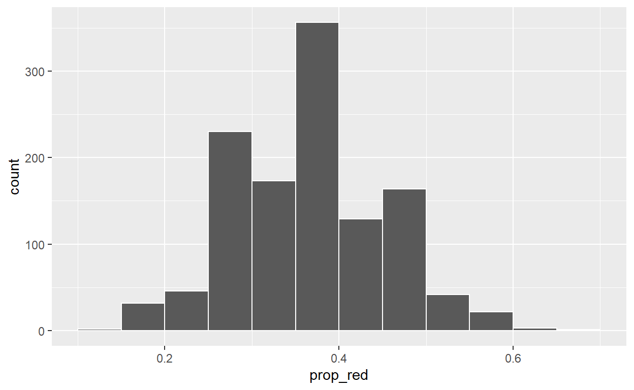
labs(x = "Proportion of 30 balls that were red", title = "30")

$x
[1] "Proportion of 30 balls that were red"

$title
[1] "30"

attr(,"class")
[1] "labels"

Segment 2: sample size = 55

2.a) Take 1200 samples of size 55 instead of 1000 replicates of size 50. Assign the output to virtual_samples_55

virtual_samples_55  <- bowl  %>% 
  rep_sample_n(size = 55, reps = 1200)

2.b) Compute resulting 1200 replicates of proportion red - start with virtual_samples_55 THEN - group_by replicate THEN - create variable red equal to the sum of all the red balls - create variable prop_red equal to variable red / 55 - Assign the output to virtual_prop_red_55

virtual_prop_red_55 <- virtual_samples_55  %>% 
  group_by(replicate) %>% 
  summarize(red = sum(color == "red")) %>% 
  mutate(prop_red = red / 55)

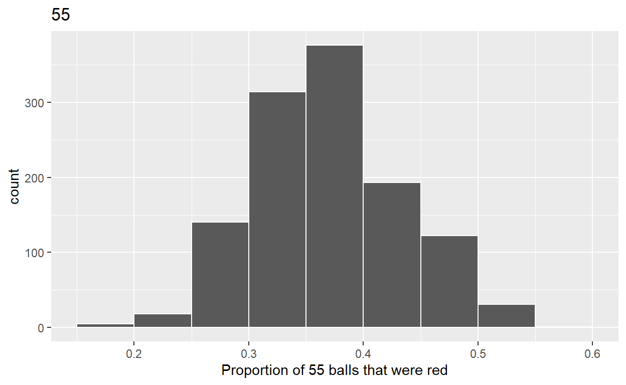
2.c) Plot distribution of virtual_prop_red_55 via a histogram use labs to - label x axis = “Proportion of 55 balls that were red” - create title = “55”

ggplot(virtual_prop_red_55, aes(x = prop_red)) +
  geom_histogram(binwidth = 0.05, boundary = 0.4, color = "white") +
  labs(x = "Proportion of 55 balls that were red", title = "55")

Segment 3: sample size = 120

3.a) Take 1200 samples of size of 120 instead of 1000 replicates of size 50. Assign the output to virtual_samples_120

virtual_samples_120  <- bowl  %>% 
  rep_sample_n(size = 120, reps = 1200)

3.b) Compute resulting 1200 replicates of proportion red - start with virtual_samples_120 THEN - group_by replicate THEN - create variable red equal to the sum of all the red balls - create variable prop_red equal to variable red / 120 - Assign the output to virtual_prop_red_120

virtual_prop_red_120  <- virtual_samples_120 %>% 
  group_by(replicate) %>% 
  summarize(red = sum(color == "red")) %>% 
  mutate(prop_red = red / 120)

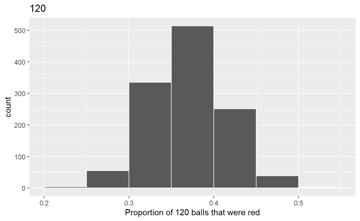
3.c) Plot distribution of virtual_prop_red_120 via a histogram use labs to - label x axis = “Proportion of 120 balls that were red” - create title = “120”

ggplot(virtual_prop_red_120, aes(x = prop_red)) +
  geom_histogram(binwidth = 0.05, boundary = 0.4, color = "white") +
  labs(x = "Proportion of 120 balls that were red", title = "120")

Calculate the standard deviations for your three sets of 1200 values of prop_red using the standard deviation

n = 30

virtual_prop_red_30 %>% 
  summarize(sd = sd(prop_red))

# A tibble: 1 x 1
      sd
   <dbl>
1 0.0865

n = 55

virtual_prop_red_55 %>% 
  summarize(sd = sd(prop_red))

# A tibble: 1 x 1
      sd
   <dbl>
1 0.0645

n = 120

virtual_prop_red_120 %>% 
  summarize(sd = sd(prop_red))

# A tibble: 1 x 1
      sd
   <dbl>
1 0.0432