Contents
Question: t-test Q: is the mean number of hours per week 48?
Question: 2 sample t-test Q: Is the average number of hours worked the same for both genders?
Question: ANOVA Q: Is the average number of hours worked the same for all three status (fired, ok and promoted)?
Load the R packages we will use.
#Question: t-test
- The data this quiz is a subset of
HR- Look at the variable definitions
- Note that the variables evaluation and salary have been recoded to be represented as words instead of numbers
- Set random seed generator to 123
set.seed(123)
hr_1_tidy.csv is the name of your data subset
- Read into and assign to
hr
hr <- read_csv("https://estanny.com/static/week13/data/hr_1_tidy.csv", col_types = "fddfff")
use the skim to summarize the data in hr
skim(hr)
| Name | hr |
| Number of rows | 500 |
| Number of columns | 6 |
| _______________________ | |
| Column type frequency: | |
| factor | 4 |
| numeric | 2 |
| ________________________ | |
| Group variables | None |
Variable type: factor
| skim_variable | n_missing | complete_rate | ordered | n_unique | top_counts |
|---|---|---|---|---|---|
| gender | 0 | 1 | FALSE | 2 | fem: 260, mal: 240 |
| evaluation | 0 | 1 | FALSE | 4 | bad: 153, fai: 142, goo: 106, ver: 99 |
| salary | 0 | 1 | FALSE | 6 | lev: 93, lev: 92, lev: 91, lev: 84 |
| status | 0 | 1 | FALSE | 3 | fir: 185, pro: 162, ok: 153 |
Variable type: numeric
| skim_variable | n_missing | complete_rate | mean | sd | p0 | p25 | p50 | p75 | p100 | hist |
|---|---|---|---|---|---|---|---|---|---|---|
| age | 0 | 1 | 40.60 | 11.58 | 20.2 | 30.37 | 41.00 | 50.82 | 59.9 | ▇▇▇▇▇ |
| hours | 0 | 1 | 49.32 | 13.13 | 35.0 | 37.55 | 45.25 | 58.45 | 79.7 | ▇▂▃▂▂ |
The mean hours worked per week is: 49.3
specify that hours is the variable of interest
hr  %>%
  specify(response = hours)
Response: hours (numeric)
# A tibble: 500 x 1
   hours
   <dbl>
 1  36.5
 2  55.8
 3  35
 4  52
 5  35.1
 6  36.3
 7  40.1
 8  42.7
 9  66.6
10  35.5
# ... with 490 more rows
hypothesize that the average hours worked is 48
hr  %>%
  specify(response = hours)  %>%
  hypothesize(null = "point", mu = 48)
Response: hours (numeric)
Null Hypothesis: point
# A tibble: 500 x 1
   hours
   <dbl>
 1  36.5
 2  55.8
 3  35
 4  52
 5  35.1
 6  36.3
 7  40.1
 8  42.7
 9  66.6
10  35.5
# ... with 490 more rows
generate 1000 replicates representing the null hypothesis
hr  %>%
  specify(response = hours)  %>%
  hypothesise(null = "point", mu = 48)  %>%
  generate(reps = 1000, type = "bootstrap")
Response: hours (numeric)
Null Hypothesis: point
# A tibble: 500,000 x 2
# Groups:   replicate [1,000]
   replicate hours
       <int> <dbl>
 1         1  33.7
 2         1  34.9
 3         1  46.6
 4         1  33.8
 5         1  61.2
 6         1  34.7
 7         1  37.9
 8         1  39.0
 9         1  62.8
10         1  50.9
# ... with 499,990 more rows
calculate the distribution of statistics from the generated data
Assign the output
null_t_distributionDisplay
null_t_distribution
null_t_distribution  <- hr %>%
  specify(response = age)  %>%
  hypothesise(null = "point", mu = 48)  %>%
  generate(reps = 1000, type = "bootstrap")  %>%
  calculate(stat = "t")

null_t_distribution
# A tibble: 1,000 x 2
replicate stat
* <int> <dbl>
1 1 0.802
2 2 -0.706
3 3 1.33
4 4 -0.245
5 5 -1.11
6 6 0.382
7 7 -0.904
8 8 0.816
9 9 0.968
10 10 0.979
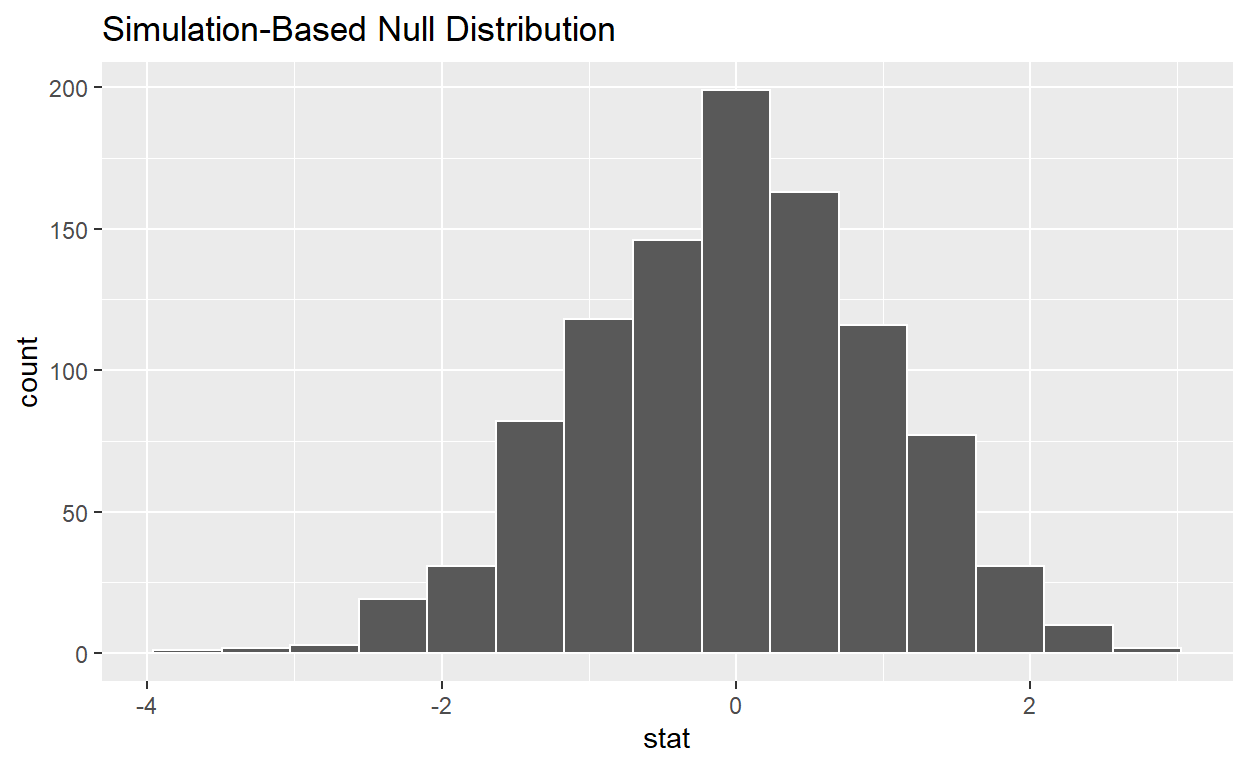
# ... with 990 more rowsvisualize the simulated null distribution
visualise(null_t_distribution)
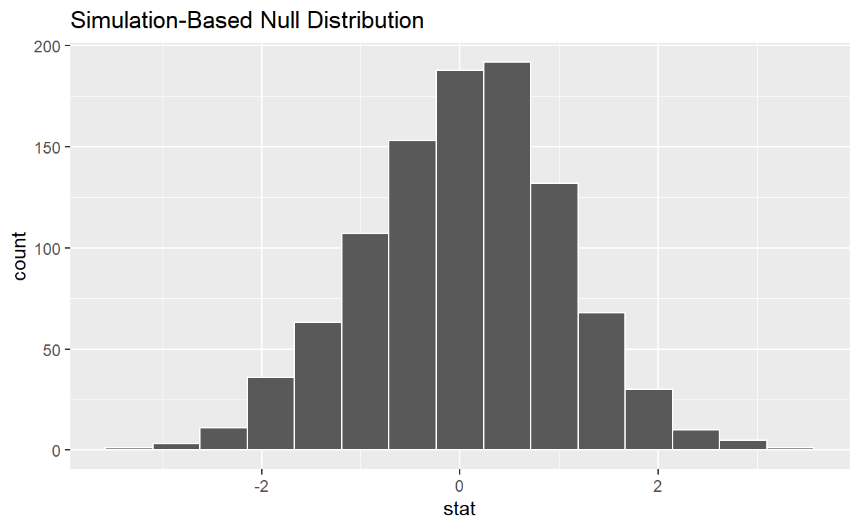
calculate the statistic from your observed data - Assign the output observed_t_statistic - Display observed_t_statistic
observed_t_statistic  <- hr  %>%
  specify(response = hours)  %>%
  hypothesize(null = "point", mu = 48)  %>%
  calculate(stat = "t")

observed_t_statistic
# A tibble: 1 x 1
stat
<dbl>
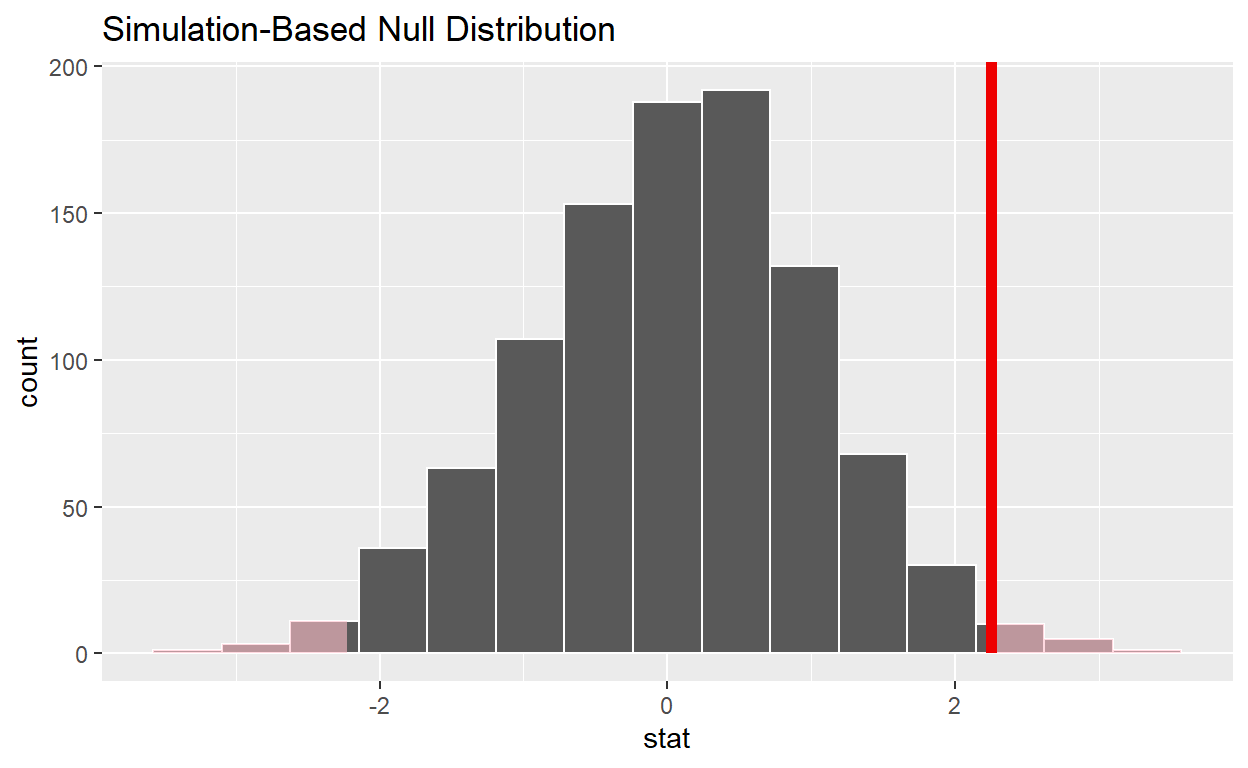
1 2.25get_p_value from the simulated null distribution and the observed statistic
null_t_distribution  %>%
  get_p_value(obs_stat = 2.25, direction = "two-sided")
# A tibble: 1 x 1
p_value
<dbl>
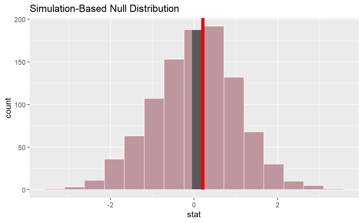
1 0.022shade_p_value on the simulated null distribution
null_t_distribution  %>%
  visualise() +
  shade_p_value(obs_stat = 2.25, direction = "two-sided")
#Question 2: sample t-test
hr_3_tidy.csv is the name of your data subset
- read it into and assign to
hr_2
hr_2 <- read_csv("https://estanny.com/static/week13/data/hr_3_tidy.csv", col_types = "fddfff")
#Q: Is the average number of hours worked the same for both genders in hr_2?
*use skim to summarize the data in hr_2 by gender
hr_2 %>%
  group_by(gender)  %>%
  skim()
| Name | Piped data |
| Number of rows | 500 |
| Number of columns | 6 |
| _______________________ | |
| Column type frequency: | |
| factor | 3 |
| numeric | 2 |
| ________________________ | |
| Group variables | gender |
Variable type: factor
| skim_variable | gender | n_missing | complete_rate | ordered | n_unique | top_counts |
|---|---|---|---|---|---|---|
| evaluation | male | 0 | 1 | FALSE | 4 | bad: 72, fai: 67, goo: 61, ver: 47 |
| evaluation | female | 0 | 1 | FALSE | 4 | bad: 76, fai: 71, goo: 61, ver: 45 |
| salary | male | 0 | 1 | FALSE | 6 | lev: 47, lev: 43, lev: 43, lev: 42 |
| salary | female | 0 | 1 | FALSE | 6 | lev: 51, lev: 46, lev: 45, lev: 43 |
| status | male | 0 | 1 | FALSE | 3 | fir: 98, pro: 81, ok: 68 |
| status | female | 0 | 1 | FALSE | 3 | fir: 98, pro: 91, ok: 64 |
Variable type: numeric
| skim_variable | gender | n_missing | complete_rate | mean | sd | p0 | p25 | p50 | p75 | p100 | hist |
|---|---|---|---|---|---|---|---|---|---|---|---|
| age | male | 0 | 1 | 38.23 | 10.86 | 20 | 28.9 | 37.9 | 47.05 | 59.9 | ▇▇▇▇▅ |
| age | female | 0 | 1 | 40.56 | 11.67 | 20 | 31.0 | 40.3 | 50.50 | 59.8 | ▆▆▇▆▇ |
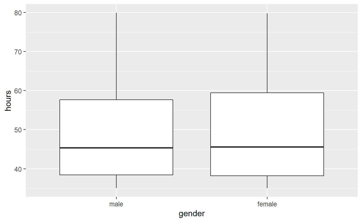
| hours | male | 0 | 1 | 49.55 | 13.11 | 35 | 38.4 | 45.4 | 57.65 | 79.9 | ▇▃▂▂▂ |
| hours | female | 0 | 1 | 49.80 | 13.38 | 35 | 38.2 | 45.6 | 59.40 | 79.8 | ▇▂▃▂▂ |
Use geom_boxplot to plot distributions of hours worked by gender
hr_2 %>%
  ggplot(aes(x = gender, y = hours)) +
  geom_boxplot()
specify the variables of interest are hours and gender
hr_2 %>%
  specify(response = hours, explanatory = gender)
Response: hours (numeric)
Explanatory: gender (factor)
# A tibble: 500 x 2
   hours gender
   <dbl> <fct>
 1  49.6 male
 2  39.2 female
 3  63.2 female
 4  42.2 male
 5  54.7 male
 6  54.3 female
 7  37.3 female
 8  45.6 female
 9  35.1 female
10  53   male
# ... with 490 more rows
hypothesize that the number of hours worked and gender are independent
hr_2 %>%
  specify(response = hours, explanatory = gender)  %>%
  hypothesise(null = "independence")
Response: hours (numeric)
Explanatory: gender (factor)
Null Hypothesis: independence
# A tibble: 500 x 2
   hours gender
   <dbl> <fct>
 1  49.6 male
 2  39.2 female
 3  63.2 female
 4  42.2 male
 5  54.7 male
 6  54.3 female
 7  37.3 female
 8  45.6 female
 9  35.1 female
10  53   male
# ... with 490 more rows
generate 1000 replicates representing the null hypothesis
hr_2 %>%
  specify(response = hours, explanatory = gender)  %>%
  hypothesize(null = "independence")  %>%
  generate(reps = 1000, type = "permute")
Response: hours (numeric)
Explanatory: gender (factor)
Null Hypothesis: independence
# A tibble: 500,000 x 3
# Groups:   replicate [1,000]
   hours gender replicate
   <dbl> <fct>      <int>
 1  55.7 male           1
 2  35.5 female         1
 3  35.1 female         1
 4  44.2 male           1
 5  52.8 male           1
 6  46   female         1
 7  41.2 female         1
 8  52.9 female         1
 9  35.6 female         1
10  35   male           1
# ... with 499,990 more rows
calculate the distribution of statistics from the generated data
- Assign the output
null_distribution_2_sample_permute - Display
null_distribution_2_sample_permute
null_distribution_2_sample_permute  <- hr_2 %>%
  specify(response = hours, explanatory = gender)  %>%
  hypothesize(null = "independence")  %>%
  generate(reps = 1000, type = "permute")  %>%
  calculate(stat = "t", order = c("female", "male"))

null_distribution_2_sample_permute
# A tibble: 1,000 x 2
   replicate    stat
 *     <int>   <dbl>
 1         1 -1.81
 2         2 -1.29
 3         3  0.0525
 4         4 -0.793
 5         5  0.826
 6         6  0.429
 7         7  0.0843
 8         8 -0.264
 9         9  2.42
10        10  0.603
# ... with 990 more rows
visualize the simulated null distribution
visualise(null_distribution_2_sample_permute)
calculate the statistic from your observed data
- Assign the output
observed_t_2_sample_stat - Display
observed_t_2_sample_stat
observed_t_2_sample_stat  <- hr_2 %>%
  specify(response = hours, explanatory = gender)  %>%
  calculate(stat = "t", order = c("female", "male"))

observed_t_2_sample_stat
# A tibble: 1 x 1
   stat
  <dbl>
1 0.208
get_p_value from the simulated null distribution and the observed statistic
null_t_distribution  %>%
  get_p_value(obs_stat = 0.208, direction = "two-sided")
# A tibble: 1 x 1
  p_value
    <dbl>
1   0.892
shade_p_value on the simulated null distribution
null_t_distribution  %>%
  visualise() +
  shade_p_value(obs_stat = 0.208, direction = "two-sided")
#Question: ANOVA
*hr_1_tidy.csv is the name of your data subset
- read it into and assign to
hr_anova
hr_anova <- read_csv("https://estanny.com/static/week13/data/hr_1_tidy.csv", col_types = "fddfff")
#Q: is the average number of hours worked the same for all three status (fired, ok, and promoted)?
use skim to summarize the data in hr_anova by status
hr_anova %>%
  group_by(status)  %>%
  skim()
| Name | Piped data |
| Number of rows | 500 |
| Number of columns | 6 |
| _______________________ | |
| Column type frequency: | |
| factor | 3 |
| numeric | 2 |
| ________________________ | |
| Group variables | status |
Variable type: factor
| skim_variable | status | n_missing | complete_rate | ordered | n_unique | top_counts |
|---|---|---|---|---|---|---|
| gender | fired | 0 | 1 | FALSE | 2 | fem: 96, mal: 89 |
| gender | ok | 0 | 1 | FALSE | 2 | fem: 77, mal: 76 |
| gender | promoted | 0 | 1 | FALSE | 2 | fem: 87, mal: 75 |
| evaluation | fired | 0 | 1 | FALSE | 4 | bad: 65, fai: 63, goo: 31, ver: 26 |
| evaluation | ok | 0 | 1 | FALSE | 4 | bad: 69, fai: 59, goo: 15, ver: 10 |
| evaluation | promoted | 0 | 1 | FALSE | 4 | ver: 63, goo: 60, fai: 20, bad: 19 |
| salary | fired | 0 | 1 | FALSE | 6 | lev: 41, lev: 37, lev: 32, lev: 32 |
| salary | ok | 0 | 1 | FALSE | 6 | lev: 40, lev: 37, lev: 29, lev: 23 |
| salary | promoted | 0 | 1 | FALSE | 6 | lev: 37, lev: 35, lev: 29, lev: 23 |
Variable type: numeric
| skim_variable | status | n_missing | complete_rate | mean | sd | p0 | p25 | p50 | p75 | p100 | hist |
|---|---|---|---|---|---|---|---|---|---|---|---|
| age | fired | 0 | 1 | 38.64 | 11.43 | 20.2 | 28.30 | 38.30 | 47.60 | 59.6 | ▇▇▇▅▆ |
| age | ok | 0 | 1 | 41.34 | 12.11 | 20.3 | 31.00 | 42.10 | 51.70 | 59.9 | ▆▆▆▆▇ |
| age | promoted | 0 | 1 | 42.13 | 10.98 | 21.0 | 33.40 | 42.95 | 50.98 | 59.9 | ▆▅▆▇▇ |
| hours | fired | 0 | 1 | 41.67 | 7.88 | 35.0 | 36.10 | 38.90 | 43.90 | 75.5 | ▇▂▁▁▁ |
| hours | ok | 0 | 1 | 48.05 | 11.65 | 35.0 | 37.70 | 45.60 | 56.10 | 78.2 | ▇▃▃▂▁ |
| hours | promoted | 0 | 1 | 59.27 | 12.90 | 35.0 | 51.12 | 60.10 | 70.15 | 79.7 | ▆▅▇▇▇ |
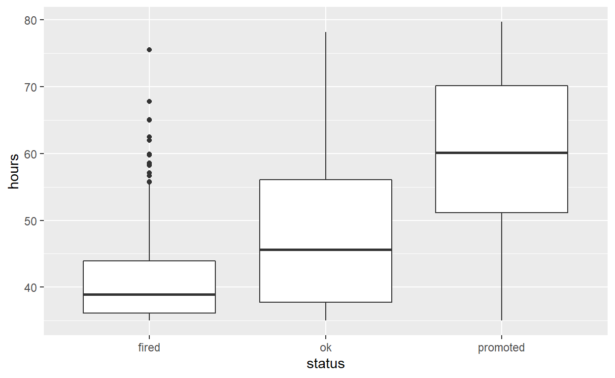
- Employees that were fired worked an average of 41.7 hours per week
- Employees that were ok worked an average of 48.0 hours per work
- Employees that were promoted worled an average of 59.3 hours per week
*Use geom_boxplot to plot distributions of hours worked by status
hr_anova %>%
  ggplot(aes(x = status, y = hours)) +
  geom_boxplot()
*specify the variables of interest are hours and status
hr_anova %>%
  specify(response = hours, explanatory = status)
Response: hours (numeric)
Explanatory: status (factor)
# A tibble: 500 x 2
   hours status
   <dbl> <fct>
 1  36.5 fired
 2  55.8 ok
 3  35   fired
 4  52   promoted
 5  35.1 ok
 6  36.3 ok
 7  40.1 promoted
 8  42.7 fired
 9  66.6 promoted
10  35.5 ok
# ... with 490 more rows
hypothesize that the number of hours worked and status are independent
hr_anova  %>%
  specify(response = hours, explanatory = status)  %>%
  hypothesise(null = "independence")
Response: hours (numeric)
Explanatory: status (factor)
Null Hypothesis: independence
# A tibble: 500 x 2
   hours status
   <dbl> <fct>
 1  36.5 fired
 2  55.8 ok
 3  35   fired
 4  52   promoted
 5  35.1 ok
 6  36.3 ok
 7  40.1 promoted
 8  42.7 fired
 9  66.6 promoted
10  35.5 ok
# ... with 490 more rows
generate 1000 replicates representing the null hypothesis
hr_anova %>%
  specify(response = hours, explanatory = status)  %>%
  hypothesise(null = "independence")  %>%
  generate(reps = 1000, type = "permute")
Response: hours (numeric)
Explanatory: status (factor)
Null Hypothesis: independence
# A tibble: 500,000 x 3
# Groups:   replicate [1,000]
   hours status   replicate
   <dbl> <fct>        <int>
 1  40.3 fired            1
 2  40.3 ok               1
 3  37.3 fired            1
 4  50.5 promoted         1
 5  35.1 ok               1
 6  67.8 ok               1
 7  39.3 promoted         1
 8  35.7 fired            1
 9  40.2 promoted         1
10  38.4 ok               1
# ... with 499,990 more rows
calculate the distribution of statistics from the generated data
- Assign the output
null_distribution_anova - Display
null_distribution_anova
null_distribution_anova  <- hr_anova %>%
  specify(response = hours, explanatory = gender)  %>%
  hypothesise(null = "independence")  %>%
  generate(reps = 1000, type = "permute")  %>%
  calculate(stat = "F")

null_distribution_anova
# A tibble: 1,000 x 2
replicate stat
* <int> <dbl>
1 1 0.365
2 2 0.650
3 3 0.185
4 4 0.0184
5 5 0.163
6 6 0.0194
7 7 4.92
8 8 2.11
9 9 0.341
10 10 0.855
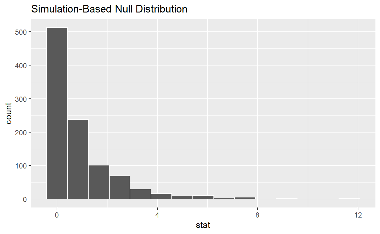
# ... with 990 more rowsvisualize the simulated null distribution
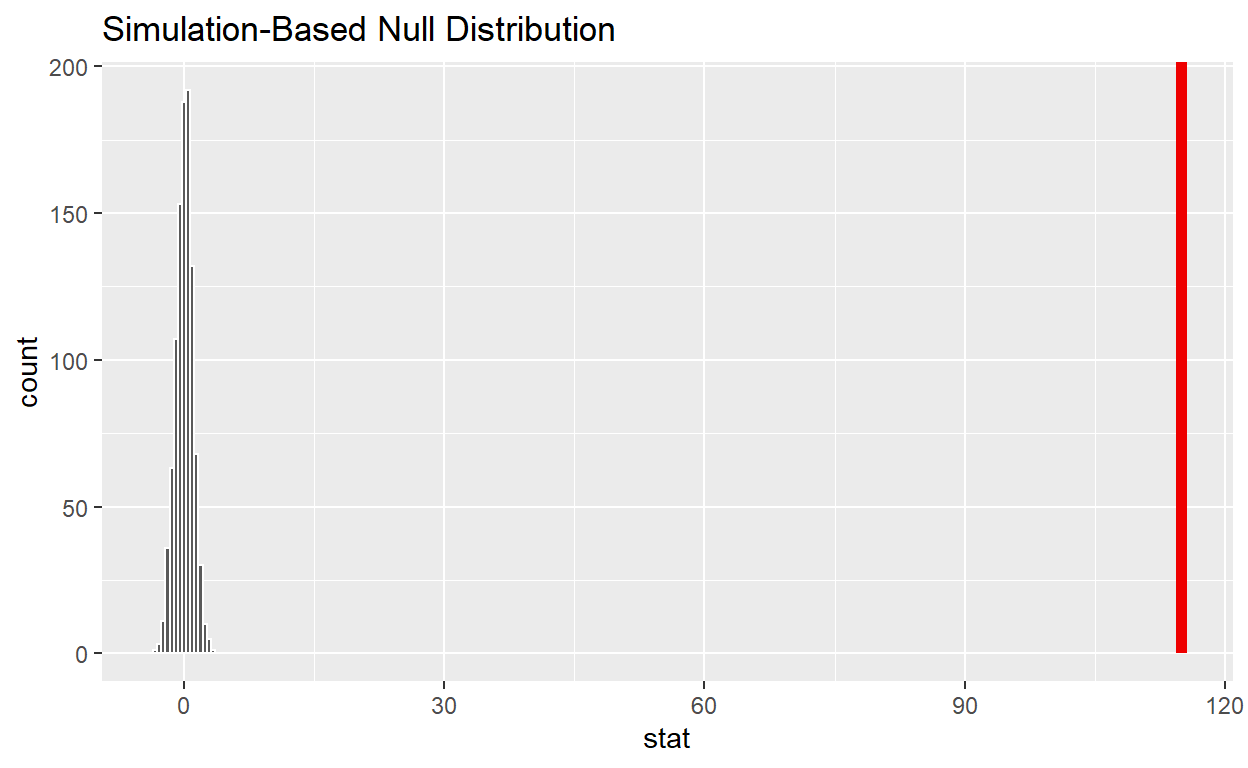
visualise(null_distribution_anova)
calculate the statistic from your observed data - Assign the output observed_f_sample_stat - Display observed_f_sample_stat
observed_f_sample_stat  <- hr_anova %>%
  specify(response = hours, explanatory = status)  %>%
  calculate(stat = "F")

observed_f_sample_stat
# A tibble: 1 x 1
   stat
  <dbl>
1  115.
get_p_value from the simulated null distribution
null_distribution_anova  %>%
  get_p_value(obs_stat = 115, direction = "greater")
# A tibble: 1 x 1
  p_value
    <dbl>
1       0
shade_p_value on the simulated null distribution
null_t_distribution  %>%
  visualise() +
  shade_p_value(obs_stat = 115, direction = "greater")